Loss Function
Regularization: Add term to loss
$L=\frac{1}{N}\sum_{i=1}^{N}\sum_{j\not= y_i}\max(0, f(x_i;W)j-f(x_i;W){y_i}+1)+\lambda R(W)$
In common use:

Dropout
In each forward pass, randomly set some neurons to zero
Probability of dropping is a hyperparameter; 0.5 is common

Data Augmentation
- Horizontal Flipping 水平翻转
- Random Cropping 随机裁剪
- Random Scaling 随机放缩
- Color Jittering 颜色抖动
- Random Translation 随机平移
- Random Shearing 随机剪切
Regression
L1 Loss
| $L(y, \hat{y})=w(\theta) | \hat{y}-y | $ |
L2 Loss
$L(y, \hat{y})=w(\theta)(\hat{y}-y)^2$
Classification
Hinge Loss Function 铰链损失函数
$L(y, \hat{y}) = \max{(0, 1-\hat{y}y)}$
$y\in{-1, 1}$
Cross-Entropy Loss Function 交叉熵损失函数
In binary classification, $L(y, \hat{y}) = -y\log{(\hat{y})}-(1-y)\log{(1-\hat{y})}$
In multiclass classification (class number = M), $L(y) = -\sum_{c=1}^My_o, c\log{(p_o, c)}$
- M - number of classes (dog, cat, fish)
- log - the natural log
- y - binary indicator (0 or 1) if class label cc is the correct classification for observation $o$
- p - predicted probability observation $o$ is of class $c$
Exponential Loss Function 指数损失函数
$L(y,\hat{y}) = \exp{(-y\hat{y})}$
SGD, Stochastic Gradient Descent 随机梯度下降
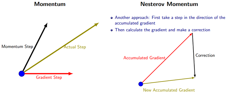
在梯度下降时,为了加快收敛速度,通常使用一些优化方法。

SGD每次都会在当前位置上沿着负梯度方向更新(下降,沿着正梯度则为上升),并不考虑之前的方向梯度大小等等。而动量(moment)通过引入一个新的变量 v去积累之前的梯度(通过指数衰减平均得到),得到加速学习过程的目的。
最直观的理解就是,若当前的梯度方向与累积的历史梯度方向一致,则当前的梯度会被加强,从而这一步下降的幅度更大。若当前的梯度方向与累积的梯度方向不一致,则会减弱当前下降的梯度幅度。
Nesterov Momentum
Ada Grad (Adaptive Gradient)
通常,我们在每一次更新参数时,对于所有的参数使用相同的学习率。而AdaGrad算法的思想是:每一次更新参数时(一次迭代),不同的参数使用不同的学习率。
Added element-wise scaling of the gradient based on the historical sum of squares in each dimension.

RMSProp: “Leaky AdaGrad”

Adam

Adam with beta1 = 0.9, beta2 = 0.999, and learning_rate = 1e-3 or 5e-4 is a great starting point for many models
Gradient Descent
1 Dimension
- Randomly pick an initial value $w^0$
-
Compute $\frac{\partial L}{\partial w} _{w=w^0}$ -
$w^1\gets w^0-\eta\frac{\partial L}{\partial w} _{w=w^0}$, where $\eta$ stands for learning rate
2 Dimension
$y=wx_1+b$
- Randomly pick an initial value $w^0, b^0$
-
Compute $\frac{\partial L}{\partial w} _{w=w^0}$, $\frac{\partial L}{\partial b} _{w=w^0, b=b^0}$ -
Update $w$ and $b$ iteratively: $w^1\gets w^0-\eta\frac{\partial L}{\partial w} _{w=w^0}$, $b^1\gets b^0-\eta\frac{\partial L}{\partial b} _{w=w^0, b=b^0}$, where $\eta$ stands for learning rate
Learning rate decay
Step
Reduce learning rate at a few fixed points. E.g. for ResNets, multiply LR by 0.1 after epochs 30, 60, and 90
Cosine
$\alpha_t=\frac{1}{2}\alpha_0(1+\cos (t\pi/T))$
- $\alpha_0$: initial learning rate
- $\alpha_t$: learning rate at epoch t
- $T$: total number of epochs
Linear
$\alpha_t=\alpha_0(1-t/T)$
Inverse Sqrt
$\alpha_t = \alpha_1/\sqrt{t}$
Looking at learning curves
Losses may be noisy, use a scatter plot and also plot moving average to see trends better.
Activation Function
introduce non-linear properties to the network

Sigmoid
Formula
\[\sigma(x) = \frac{1}{1+e^{-x}}\]Features
- Squashes numbers to range [0, 1]
Problems
-
Saturated neurons “kill” the gradients
-
Sigmoid outputs are not zero-centered
The gradient on $w$ is always all positive or negative, so the gradient can upgrade in only one direction.
-
A bit compute expensive
Tanh
Formula
\[\tanh(x) = \frac{\sinh(x)}{\cosh(x)}=\frac{e^x-e^{-x}}{e^x+e^{-x}}\]Features
- Squashes number to range [-1, 1]
- Zero centered
Problems
- Saturated neurons “kill” the gradients
ReLU
Formula
\[f(x) = \max(0, x)\]Features
- Does not saturate (in >0 region)
- Very computationally efficient
- Converges much faster
- More biologically plausible
Problems
- Not zero-centered
- “kill” the gradients (in $\le$ 0 region), what we called the “dead ReLU”
Leaky ReLU
Formula
\[f(x) = \max(0.01x, x)\]Features
- Does not saturate (in >0 region)
- Vary computationally efficient
- Converges much faster
- Will not “die”
References
Parametric Rectifier (PReLU)
\[f(x) = \max(\alpha x, x)\]ELU
Formula
\[f(x) = \left\{ \begin{array}{lc} x & if\ x > 0\\\alpha(\exp{(x)}-1) & if\ x \le 0\end{array}\right.\]Features
- All benefits of ReLU
- Closer to zero mean outputs
- Negative saturation regime compared with Leaky ReLU adds some robustness to noise
Problems
- Computation requires exp()
Maxout
There is also another popular variant called maxout which is the generalized form above relu and leaky relu.
Formula
\[\max(w_1^T x+b_1, w_2^T x+b_2)\]Features
- Generalizes ReLU and Leaky ReLU
- Does not saturate
- Does not die
Problems
- Doubles the number of parameters / neuron
Layers
Fully Connected Layer
dot product

Convolution Layer

Number of parameters in the layer: $K\times (F^2\times C + 1)$
$+1$ for bias
GANS, Generative Adversarial Network 生成对抗网络

Generative Model G 生成器
Captures data distribution and generate samples close to real distribution
Discriminative Model D 判别器
Estimates the probability that a sample came from the training data rather than G


